Linear Regression with Pytorch

Linear Regression through Pytorch

• 이번 포스트의 목적은 Linear Model을 Pytorch을 통해 구현해보며, 개인적으로 Pytorch의 사용을 연습하며 적응력을 높여보는 것입니다.

Import Library

import torch
import torch.optim as optim

import matplotlib.pyplot as plt
import numpy as np

import warnings
warnings.filterwarnings("ignore")
%config InlineBackend.figure_format = 'retina'
%matplotlib inline

Generate Toy Data

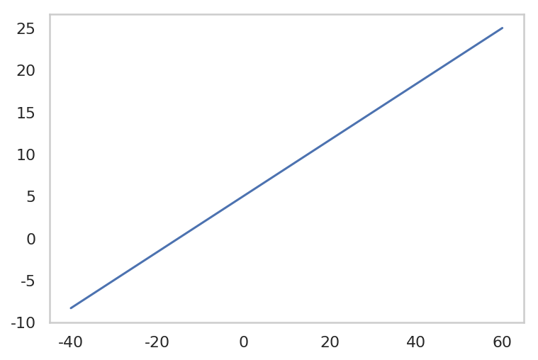
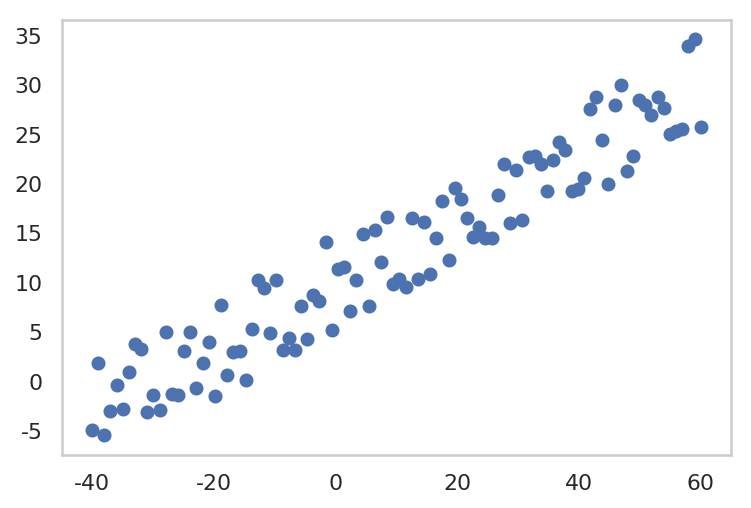
$ y = \frac{1}{3} x + 5 $ 와 약간의 noise 를 합쳐 100 개의 toy data를 만들겠습니다.

# Target Function
f = lambda x: 1.0/3.0 * x + 5.0

x = np.linspace(-40, 60, 100)
fx = f(x)

plt.plot(x, fx)
plt.grid()
plt.show()

# y_train data with little noise
y = fx + 10 * np.random.rand(len(x))

plt.plot(x, y, 'o')
plt.grid()
plt.show()

1. Gradient Descent

1. Model (hypothesis) 를 설정합니다.
   (여기선, Linear Regression 이므로, $y = Wx + b$ 형태를 사용합니다.)
2. Loss Function 을 정의합니다. (여기선, MSE loss 를 사용하겠습니다.)
3. gradient 를 계산합니다.
   (여기선, Gradient Descent 방법으로 optimize 를 할 것이므로, optim.SGD() 를 사용합니다.)
4. parameter 를 update 합니다.

x_train = torch.FloatTensor(x)
y_train = torch.FloatTensor(y)
print("x_train Tensor shape: ", x_train.shape)
print("y_train Tensor shape: ", y_train.shape)

x_train Tensor shape:  torch.Size([100])
y_train Tensor shape:  torch.Size([100])

# train code

# parameter setting & initialize
W = torch.zeros(1, requires_grad=True)
b = torch.zeros(1, requires_grad=True)

# optimizer setting
optimizer = optim.SGD([W, b], lr=0.001)

# total epochs
epochs = 3000

for epoch in range(1, epochs + 1):
    # decide model(hypothesis)
    model = W * x_train + b
    
    # loss function -> MSE
    loss = torch.mean((model - y_train)**2)
    
    optimizer.zero_grad()
    loss.backward()
    optimizer.step()
    
    # 10 epoch 마다 train loss 를 출력합니다.
    if epoch % 500 == 0:
        print("epoch: {} -- Parameters: W: {} b: {} -- loss {}".format(epoch, W.data, b.data, loss.data))

epoch: 500 -- Parameters: W: tensor([0.3709]) b: tensor([5.6408]) -- loss 22.728315353393555
epoch: 1000 -- Parameters: W: tensor([0.3467]) b: tensor([7.9427]) -- loss 11.399767875671387
epoch: 1500 -- Parameters: W: tensor([0.3368]) b: tensor([8.8829]) -- loss 9.51008415222168
epoch: 2000 -- Parameters: W: tensor([0.3327]) b: tensor([9.2669]) -- loss 9.194862365722656
epoch: 2500 -- Parameters: W: tensor([0.3311]) b: tensor([9.4237]) -- loss 9.142287254333496
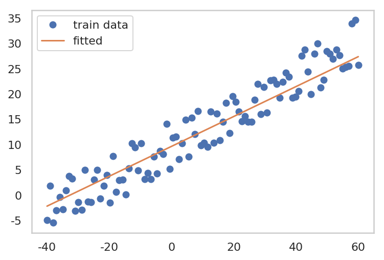
epoch: 3000 -- Parameters: W: tensor([0.3304]) b: tensor([9.4878]) -- loss 9.133516311645508

plt.plot(x, y, 'o', label="train data")
plt.plot(x_train.data.numpy(), W.data.numpy()*x + b.data.numpy(), label='fitted')
plt.grid()
plt.legend()
plt.show()

2. Stochastic Gradient Descent

1. Model (hypothesis) Setting
2. Loss Function Setting
3. 최적화 알고리즘 선택
4. shuffle train data
5. mini-batch 마다 W, b 업데이트

# batch 를 generate 해주는 함수
def generate_batch(batch_size, x_train, y_train):
    assert len(x_train) == len(y_train)
    result_batches = []
    x_size = len(x_train)
    
    shuffled_id = np.arange(x_size)
    np.random.shuffle(shuffled_id)
    shuffled_x_train = x_train[shuffled_id]
    shuffled_y_train = y_train[shuffled_id]
    
    for start_idx in range(0, x_size, batch_size):
        end_idx = start_idx + batch_size
        batch = [shuffled_x_train[start_idx:end_idx], shuffled_y_train[start_idx:end_idx]]
        result_batches.append(batch)
    return result_batches

# train
W = torch.zeros(1, requires_grad=True)
b = torch.zeros(1, requires_grad=True)

optimizer = optim.SGD([W, b], lr=0.001)

epochs = 10000

for epoch in range(1, epochs + 1):
    for x_batch, y_batch in generate_batch(10, x_train, y_train):
        model = W * x_batch + b
        loss = torch.mean((model - y_batch)**2)
        
        optimizer.zero_grad()
        loss.backward()
        optimizer.step()
        
    if epoch % 500 == 0:
        print("epoch: {} -- Parameters: W: {} b: {} -- loss {}".format(epoch, W.data, b.data, loss.data))

epoch: 500 -- Parameters: W: tensor([0.0890]) b: tensor([9.5399]) -- loss 162.1055450439453
epoch: 1000 -- Parameters: W: tensor([0.3672]) b: tensor([9.5366]) -- loss 12.424881935119629
epoch: 1500 -- Parameters: W: tensor([0.3560]) b: tensor([9.5097]) -- loss 7.826609134674072
epoch: 2000 -- Parameters: W: tensor([0.3375]) b: tensor([9.5556]) -- loss 13.15934944152832
epoch: 2500 -- Parameters: W: tensor([0.2462]) b: tensor([9.5157]) -- loss 11.582895278930664
epoch: 3000 -- Parameters: W: tensor([0.3097]) b: tensor([9.5111]) -- loss 9.991677284240723
epoch: 3500 -- Parameters: W: tensor([0.2497]) b: tensor([9.5532]) -- loss 20.481367111206055
epoch: 4000 -- Parameters: W: tensor([0.4388]) b: tensor([9.5390]) -- loss 20.827198028564453
epoch: 4500 -- Parameters: W: tensor([0.1080]) b: tensor([9.4959]) -- loss 140.0277862548828
epoch: 5000 -- Parameters: W: tensor([0.3188]) b: tensor([9.4829]) -- loss 6.635367393493652
epoch: 5500 -- Parameters: W: tensor([0.2553]) b: tensor([9.5017]) -- loss 25.45773696899414
epoch: 6000 -- Parameters: W: tensor([0.2490]) b: tensor([9.5489]) -- loss 9.580666542053223
epoch: 6500 -- Parameters: W: tensor([0.3189]) b: tensor([9.5347]) -- loss 12.585128784179688
epoch: 7000 -- Parameters: W: tensor([0.3026]) b: tensor([9.4874]) -- loss 8.298829078674316
epoch: 7500 -- Parameters: W: tensor([0.3507]) b: tensor([9.6815]) -- loss 13.348054885864258
epoch: 8000 -- Parameters: W: tensor([0.1423]) b: tensor([9.5220]) -- loss 32.567440032958984
epoch: 8500 -- Parameters: W: tensor([0.7147]) b: tensor([9.5182]) -- loss 75.97190856933594
epoch: 9000 -- Parameters: W: tensor([0.5170]) b: tensor([9.5289]) -- loss 39.07848358154297
epoch: 9500 -- Parameters: W: tensor([0.3748]) b: tensor([9.5590]) -- loss 10.358983993530273
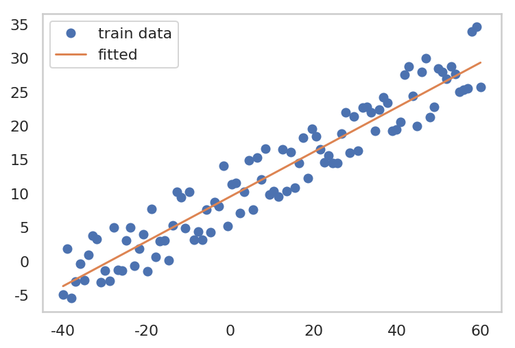
epoch: 10000 -- Parameters: W: tensor([0.2958]) b: tensor([9.6088]) -- loss 7.410649299621582

• Stochasitic 하게 loss의 gradient 를 계산하여, parameter update를 하므로, loss 가 굉장히 oscilation 이 나타나며 감소하는 것을 볼 수 있다.

plt.plot(x, y, 'o', label="train data")
plt.plot(x_train.data.numpy(), W.data.numpy()*x + b.data.numpy(), label='fitted')
plt.grid()
plt.legend()
plt.show()